Linear Regression from Scratch

Linear regression is one of the simplest machine learning algorithms and is the best practice for beginners. In this post I will guide you step by step creating a Linear Regression model from scratch.

---

What is Linear Regression?

Let’s start with some data. Suppose we measured different car models and collected some data with respect to their fuel effeciency and engine size. (If you wonder, this is the mtcars dataset in R language.) Let’s load the data and shows the first 5 rows of the data, in which mpg is the fuel efficiency in Miles per Gallon and disp is the engine size in cu.in. :

import pandas as pd
import numpy as np
import matplotlib.pyplot as plt

df = pd.read_csv('https://gist.githubusercontent.com/seankross/a412dfbd88b3db70b74b/raw/5f23f993cd87c283ce766e7ac6b329ee7cc2e1d1/mtcars.csv')
df[['model', 'disp', 'mpg']].head()

	model	disp	mpg
0	Mazda RX4	160.0	21.0
1	Mazda RX4 Wag	160.0	21.0
2	Datsun 710	108.0	22.8
3	Hornet 4 Drive	258.0	21.4
4	Hornet Sportabout	360.0	18.7

We can plot disp and mpg as Figure 1.

plt.scatter(x=df.disp, y=df.mpg, marker='o')
plt.xlabel('Engine Size (cubic inches)')
plt.ylabel('Fuel Effeciency (Miles per Gallon)')
plt.title('Fuel Efficiency From the `mtcars` Dataset')
plt.show()

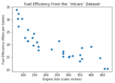
Now we need a model which outputs the fuel effeciency given the engine size as input. Why? Because if we have a new engine for which we want to know the efficiency, the plot in Figure 1 will not help.

One of the simplest models is called Linear Regresion model, or a straight line in the form of \(y = wx + b\), in which \(w, b\) are coefficients. Intuitively we can draw the line as Figure 2.

plt.scatter(x=df.disp, y=df.mpg, marker='o')
plt.xlabel('Engine Size (cubic inches)')
plt.ylabel('Fuel Effeciency (Miles per Gallon)')
plt.title('Fuel Efficiency From the `mtcars` Dataset')
x = np.linspace(0, 500)
y = -0.05 * x + 30.0
plt.plot(x, y, '--', color='r')
plt.show()

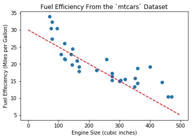
The equation for the line above is \(y = -0.05x + 30.0\). With this model, we can compute efficiency for any new engine. For example given engine size 200 cu.in., we can predict that fuel effeciency is \(-0.05 \times 200 + 30.0 = 20.0 mpg\).

Error, or Loss

You may want to ask: is \(y = -0.05x + 30.0\) the correct answer? Since most of the given data points are not on this line (practically it is impossible to draw a straight line across all the points), we could alternatively ask: Is this the best line we can draw? Or, how good is this model for prediction?

We need a measurement of the “accuracy” of this model. For each data point we have, we compute the difference between the actual effeciency and the predict effeciency from the model. In math language, we compute:

$$y – \hat{y} = y – (-0.05x + 30.0)$$

In which \(\hat{y}\) pronounces “y hat” and denotes the effeciency predicted by the model given x (engine size). Then we compute the summation of the squared difference for all the data points. The reason for taking square is to prevent positive and negative numbers from cancelling each other.

We also added 1/2 to the equation to make future numerical computation easier.

$$ \begin{align*}L &= \frac{1}{2n}\big((y_1 – \hat{y}_1)^2 + (y_2 – \hat{y}_2)^2 + \cdots + (y_n – \hat{y}_n)^2\big) \\
&= \frac{1}{2n}\sum_{i=1}^n (y_i – \hat{y}_i)^2.
\end{align*}
$$

This \(L\), called “loss”, or “error”, is the measurement of the accuracy of the model. The formula we used here is called “MSE” (Mean Squared Error).

Now let us compute the error:

np.mean(np.square(df.mpg - (-0.05 * df.disp + 30.0)))

13.705833593749997

Minimize Loss

In order to find the optimal model, we want the loss to be minimal. Let us take a look at the equation of the loss function:

$$L = \frac{1}{2n} \sum_{i=1}^n (y_i – \hat{y}_i) ^ 2 = \frac{1}{2n}\sum_{i=1}^n (y_i – (wx_i + b)) ^ 2 $$

Our goal is to find the optimal line, or coefficients \(w, b\), by minimize loss \(L\). In this task, \(x_i, y_i\) are the data points provided by our mtcars data, which we called training data. So our goal can be represented as:

$$
\begin{align}
&\text{Given training data }\mathcal{D} = \{ (x_1, y_1), (x_2, y_2), \cdots, (x_n, y_n) \}, \\
&\text{find }w, b \text{ to minimize }L.
\end{align}
$$

Note that the variables in above problem are \(w, b\), not \(x_i, y_i\)!

This function is a convex function (proof is out of scope), so to find the minimum, we only need to take the partial derivative with respect to \(w, b\) and let them equal to zero, then solve the coefficients \(w, b\).

Here is the step-by-step solution:

$$
\begin{align*}
\frac{\partial E}{\partial w} &= \frac{\partial}{\partial w} \frac{1}{2n}\sum (y_i – (wx_i + b)) ^ 2
= \frac{1}{2n} \sum \frac{\partial}{\partial w}\big(y_i – (wx_i + b)\big)^2 \\
&= \frac{1}{2n} \sum 2 (y_i – wx_i – b)(-x_i)
= \frac{1}{n} \sum (wx_i + b – y_i) \cdot x_i, \\
\\
\frac{\partial E}{\partial b} &= \frac{\partial}{\partial b} \frac{1}{2n}\sum (y_i – (wx_i + b)) ^ 2
= \frac{1}{2n} \sum \frac{\partial}{\partial b}\big(y_i – (wx_i + b)\big)^2 \\
&= \frac{1}{2n} \sum 2 (y_i – wx_i – b)(-1)
= \frac{1}{n} \sum (wx_i + b – y_i). \\
\end{align*}
$$

Let both equal to zero, we have

$$
\frac{\partial E}{\partial w} = \frac{1}{n} \sum (wx_i + b – y_i) \cdot x_i = 0,\\
\frac{\partial E}{\partial w} = \frac{1}{n} \sum (wx_i + b – y_i) = 0.
$$

Solve this equation system we have

$$
w = \frac{n \sum x_iy_i – \sum x_i \sum y_i}{n \sum x_i^2 – \big(\sum x_i \big) ^2}, \;
b = \frac{1}{n}\big(\sum y_i – w \sum x_i).
$$

The following code will compute \(w, b\) for us:

n = len(df)
x = df.disp
y = df.mpg
sum_x = np.sum(x)
sum_y = np.sum(y)
sum_xy = np.sum(x * y)
sum_x2 = np.sum(x * x)

w = (n * sum_xy - sum_x * sum_y) / (n * sum_x2 - sum_x * sum_x)
b = (sum_y - w * sum_x) / n
print(w, b)

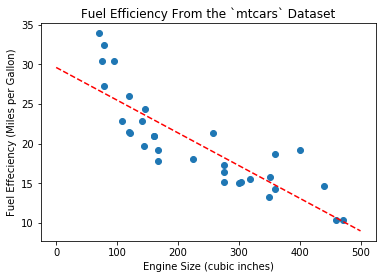
-0.041215119962786144 29.59985475616395

These are the optimal coefficients for \(w, b\) and the line equation is \(y = -0.041215 x + 29.5999\). We can plot the line with these new coefficients, as in Figure 3:

Linear Regression in Matrix Form

In previous section we saw that computing the partial derivatives with respect to \(w, b\) involves pretty complicated mathmatics. Fortunately, we can use vectors and matrices to make the calculation easier.

First, let us rewrite the line equation \(y = wx + b\) as this form:

$$ y = \begin{bmatrix}1 & x\end{bmatrix} \begin{bmatrix} b \\ w\end{bmatrix} $$

This is a trick to merge \(w, b\) into one vector variable so that we don’t need to compute partial derivates twice.

Denote \(\begin{bmatrix}b & w\end{bmatrix}^\intercal\) as \(\mathbf{w}\) and \(\begin{bmatrix}1 & x \end{bmatrix}^\intercal\) as \(\mathbf{x}\) (use bold letters to show they are vectors), then the equation can be written as:

$$ y = \mathbf{x}^\intercal \mathbf{w} $$

Now we consider all the data points \((x_i, y_i), \forall i \in \{1 \cdots n\} \). The loss function can be written as:

$$
\begin{align}
L &= \frac{1}{2n}\sum_{i=1}^n (y_i – \hat{y}_i)^2 \\
&= \frac{1}{2n} \big((y_1 – \hat{y}_1)^2 + \cdots + (y_n – \hat{y}_n)^2\big) \\
&= \frac{1}{2n} \lVert \mathbf{y} – \hat{\mathbf{y}} \rVert ^ 2 \\
&= \frac{1}{2n} \lVert \mathbf{y} – \mathbf{X}\mathbf{w} \rVert ^ 2.
\end{align}
$$

Here we used some vector and matrix notations:

$$ \mathbf{y} = \begin{bmatrix}y_1 \\ y_2 \\ \vdots \\ y_n\end{bmatrix}, \;
\mathbf{X} = \begin{bmatrix}\mathbf{x}_1^\intercal \\ \mathbf{x}_2^\intercal \\ \vdots \\ \mathbf{x}_n^\intercal \end{bmatrix}
= \begin{bmatrix}1 & x_1 \\ 1 & x_2 \\ \vdots & \vdots \\ 1 & x_n \end{bmatrix}.
$$

And the notation \(\lVert \cdot \rVert\) is the \(L^2\) norm. Thus \(\lVert \mathbf{y} – \hat{\mathbf{y}} \rVert ^ 2 = \sum (y_i – \hat{y}_i)^2 \), and it is easy to validate that this equation is equavilent to the one we used in previous section.

Next, we use the same approach to find the minimal loss by letting the gradient (the vector consists of partial derivatives of each component) equal to zero. To compute the gradient, we write the equation as:

$$
\begin{align}
L &= \frac{1}{2n} \lVert \mathbf{y} – \mathbf{Xw} \rVert ^ 2
= \frac{1}{2n} (\mathbf{y} – \mathbf{Xw})^\intercal (\mathbf{y} – \mathbf{Xw}) \\
&= \frac{1}{2n} \big(
\mathbf{y}^\intercal \mathbf{y} –
\mathbf{y}^\intercal \mathbf{Xw} –
(\mathbf{Xw})^\intercal \mathbf{y} +
(\mathbf{Xw})^\intercal (\mathbf{Xw})
\big) \\
&= \frac{1}{2n} \big(
\mathbf{y}^\intercal \mathbf{y} –
2 \mathbf{w}^\intercal \mathbf{X}^\intercal \mathbf{y} +
\mathbf{w}^\intercal \mathbf{X}^\intercal \mathbf{Xw}
\big).
\end{align}
$$

Now we compute its gradient.

$$
\begin{align}
\nabla_w L = \frac{1}{2n} \nabla_w \big(\mathbf{y}^\intercal \mathbf{y} –
2 \mathbf{w}^\intercal \mathbf{X}^\intercal \mathbf{y} +
\mathbf{w}^\intercal \mathbf{X}^\intercal \mathbf{Xw}
\big) = 0.
\end{align}
$$

To calculate the gradient with respect to \(\mathbf{w}\):

• The first term \(\mathbf{y}^\intercal \mathbf{y}\) is constant with respect to \(\mathbf{w}\), thus the gradient is 0;
• The gradient of the second term \(-2 \mathbf{w}^\intercal \mathbf{X} ^\intercal \mathbf{y}\) is \(-2 \mathbf{X}^\intercal \mathbf{y}\);
• The gradient of the third term \(\mathbf{w}^\intercal \mathbf{X}^\intercal \mathbf{Xw}\) is \(2\mathbf{X}^\intercal \mathbf{Xw}\).

Thus the gradient of loss is:

$$
\begin{align}
& 0 – 2\mathbf{X}^\intercal \mathbf{y} + 2\mathbf{X}^\intercal \mathbf{Xw} = 0. \\
&\Rightarrow \mathbf{X}^\intercal \mathbf{Xw} = \mathbf{X}^\intercal \mathbf{y}. \\
&\Rightarrow \mathbf{w} = \big(\mathbf{X}^\intercal \mathbf{X}\big)^{-1} \mathbf{X}^\intercal \mathbf{y}.
\end{align}
$$

This is the analytic solution for the linear regression model. We can use this equation to find the optimal model:

n = len(df)
X = np.vstack([np.ones([n]), df.disp]).T
y = df.mpg
# @ is a new operator in Python 3 for matrix multiplication
w = np.linalg.inv(X.T @ X) @ X.T @ y
print(w)

array([29.59985476, -0.04121512])

We got the same results as previous section, with only one line of code!

Matrix form is very useful and makes calculation much easier, especially for multivariant linear regression model, which we will cover in the next section.

Multivariant Linear Regression

We just explained how to build a linear regression model to predict fuel efficiency from engine size. However, fuel effeciency is a complex phenomenon that may have many contributing factors other than engine size, so when creating linear regression model, using more factors may result in a more robust model. Here the “contributing factors” are called features. The linear model we just discussed includes only one feature disp. In order to consider multiple features, we need to implement multivariant linear regression.

The linear regression model we used in previous section was simply a straight line in 2-D space:

$$y = wx + b$$

Here \(x\) is the input feature and \(y\) is the predicted output. In order to use multiple features, we simply change the equation to this form:

$$y = b + w_1 x_1 + w_2 x_2 + \cdots + w_d x_d$$

where \(x_1, x_2, \cdots\) are input features, and \(d\) is the number of features. This equation is a hyperplane in a \(d+1\) dimension space.

Since \(b, w_1, w_2, \cdots\) are all coefficients, we generally write \(b\) as \(w_0\), and add a dummy input \(x_0 = 1\) which is a constant, to get a more generic equation:

$$
\begin{align}
y &= w_0 x_0 + w_1 x_1 + w_2 x_2 + \cdots + w_d x_d \\
\text{Input: } \mathbf{x} &= (x_0 = 1, x_1, x_2, \cdots, x_d) \in \mathbb{R}^{d+1} \\
\text{Model Parameters}: \mathbf{w} &= (w_0, w_1, w_2, \cdots, w_d) \in \mathbb{R}^{d+1}
\end{align}
$$

This can be written in vector form:

$$ y = \mathbf{x}^\intercal \mathbf{w}$$

Now we consider multiple training data points \(\mathcal{D} = \{ (\mathbf{x}_1, y_1), \cdots, (\mathbf{x}_n, y_n) \}\). Using the following notation:

$$ \mathbf{y} = \begin{bmatrix}y_1 \\ y_2 \\ \vdots \\ y_n\end{bmatrix}, \;
\mathbf{X} = \begin{bmatrix}\mathbf{x}_1^\intercal \\ \mathbf{x}_2^\intercal \\ \vdots \\ \mathbf{x}_n^\intercal \end{bmatrix}
= \begin{bmatrix}1 & x_{11} & x_{12} & \cdots & x_{1d} \\
1 & x_{21} & x_{22} & \cdots & x_{2d} \\
\vdots & \vdots & \vdots & \ddots & \vdots \\
1 & x_{n1} & x_{n2} & \cdots & x_{nd} \end{bmatrix},
$$

We can write the linear regression model as:

$$\mathbf{y} = \mathbf{Xw}.$$

Now we can use the same procedure in previous post to find the analytic solution for this equation:

$$\mathbf{w} = \big(\mathbf{X}^\intercal \mathbf{X}\big)^{-1} \mathbf{X}^\intercal \mathbf{y}.$$

With this equation we can easily make a multivariant linear regression model:

import pandas as pd
import numpy as np

df = pd.read_csv('https://gist.githubusercontent.com/seankross/a412dfbd88b3db70b74b/raw/5f23f993cd87c283ce766e7ac6b329ee7cc2e1d1/mtcars.csv')

n = len(df)
columns = ['cyl', 'disp', 'hp', 'drat', 'wt', 'qsec', 'vs', 'am', 'gear', 'carb']

y = df['mpg']
X = df[columns]

# Add x_0 for each x
X = np.hstack([np.ones([n, 1]), X])

w = np.linalg.inv(X.T @ X) @ X.T @ y
print(w)

The output is:

[12.30337416 -0.11144048  0.01333524 -0.02148212  0.78711097 -3.71530393
  0.82104075  0.31776281  2.52022689  0.65541302 -0.19941925]

This means the equation of the model is:

$$
\begin{align}
y = &12.30337416 – 0.11144048 \cdot \text{cyl} + 0.01333524 \cdot \text{disp} – 0.02148212 \cdot \text{hp} + \\
& 0.78711097 \cdot \text{drat} – 3.71530393 \cdot \text{wt} + 0.82104075 \cdot \text{qsec} + 0.31776281 \cdot \text{vs} + \\
&2.52022689 \cdot \text{am} + 0.65541302 \cdot \text{gear} – 0.19941925 \cdot \text{carb}.
\end{align}
$$

---

Thanks for reading, and I hope this article has explained the details of the simplest linear regression model!

---

Originally posted at https://hackernoon.com/linear-regression-from-scratch-1c22ff292592.